Introduction

WarningTo do

These pages are under development.

While the provides an incredibly accurate description of the most fundamental constituents of matter, it remains difficult to describe interactions at the level of bound states (). This is because the fundamental force that dominates at this range―the ―is characterized by an : it has a strong coupling constant at low momentum transfer.

One the one hand, this asymptotic behavior of the strong force forces to bound together in colorless groups (), giving particle physicists an amazingly varied spectrum of quark combinations to study. On the other, the asymptotic running of the coupling constant makes it almost impossible to predict from first principles how bound states of quarks interact at lower energies.

Theoreticians have developed several descriptive models and numerical tools ( most importantly), but these models often rest on several assumptions or fail to describe larger systems. It therefore remains important to study particle interactions at the lower energies.

Partial Wave Analysis is a collection of techniques that allows us to perform these studies.

WarningTo do

• Importance of decomposing interactions
• Strong QCD coupling constant at low momentum transfer
• Cannot compute intermediate states from theory
• Need to collect properties: mass, width, spin, parity`

Scattering theory

Tip

An extensive, chronological lists of publications on scattering theory can be found here.

Transition amplitude

WarningTo do

• Amplitudes and intensities
• Scattering operator \(S\) ()
• Lead-up to \(T\)-matrix ()
• Distinction dynamical part and angular part

Partial waves

WarningTo do

Decomposition into partial waves [1], p.3:

Consider an incident wave \(\left|i\right> = Psi_i\). In an experimental setting, we can assume a vanishing potential at \(t\rightarrow\infty\), which allows us to expand the incoming wave in terms of Legendre polynomials \(P_l\), with \(l\) the angular orbital momentum:

\[ \Psi{=tex}*i(r,\theta{=tex}) = \sum{=tex}*{l=0}\^\infty {=tex}U_l(r) P_l(\theta{=tex}) \]

The \(U_l\) factor can be parametrized further. At this stage, it is important to point that the angular orbital momentum of the incoming state is used to characterize specific systems. Here, it is common to use the labels used for electron orbitals:

\(l\) Label Origin

---

0 s “sharp” 1 p “principal” 2 d “diffuse” 3 f “fundamental” 4 g rest is alphabetical … … …

In PWA, it is therefore common to distinguish these wave contributions as \(S\)-wave, \(P\)-wave, etc.

WarningTo do

• Separating out angular and radial wave functions using Legendre polynomials
• What we can see from this and how it relates to analysis techniques
• (?) Difference with amplitude analysis
• Possible initial states: 1, 2, and multi-body
• Suitable for propagation, not re-scattering

Isobar model

Mandelstam variables

import matplotlib.pyplot as plt
from feynman import Diagram

fig, ax = plt.subplots(1, 3, figsize=(9, 3), frameon=False, tight_layout=True)
fig.patch.set_visible(False)
for a in ax:
    a.axis("off")
    a.set_xlim(0, 1)
    a.set_ylim(0, 0.8)

s_channel = Diagram(ax[0])
# Vertices
v_p1 = s_channel.vertex(xy=(0.1, 0.7), marker="")
v_p2 = s_channel.vertex(tuple(v_p1.xy), dy=-0.6, marker="")
v_p3 = s_channel.vertex(tuple(v_p1.xy), dx=0.8, marker="")
v_p4 = s_channel.vertex(tuple(v_p3.xy), dy=-0.6, marker="")
v1 = s_channel.vertex(tuple(v_p1.xy), dx=0.2, dy=-0.3, marker="")
v2 = s_channel.vertex(tuple(v_p3.xy), dx=-0.2, dy=-0.3, marker="")
# Lines
p1 = s_channel.line(v_p1, v1, arrow=False)
p2 = s_channel.line(v1, v_p2, arrow=False)
interaction = s_channel.line(v1, v2, style="dotted", arrow=False)
e4 = s_channel.line(v2, v_p3, arrow=False)
e5 = s_channel.line(v_p4, v2, arrow=False)
# Labels
v_p1.text("$p_1$", x=-0.06, y=0)
v_p2.text("$p_2$", x=-0.06, y=0)
v_p3.text("$p_3$", x=+0.06, y=0)
v_p4.text("$p_4$", x=+0.06, y=0)
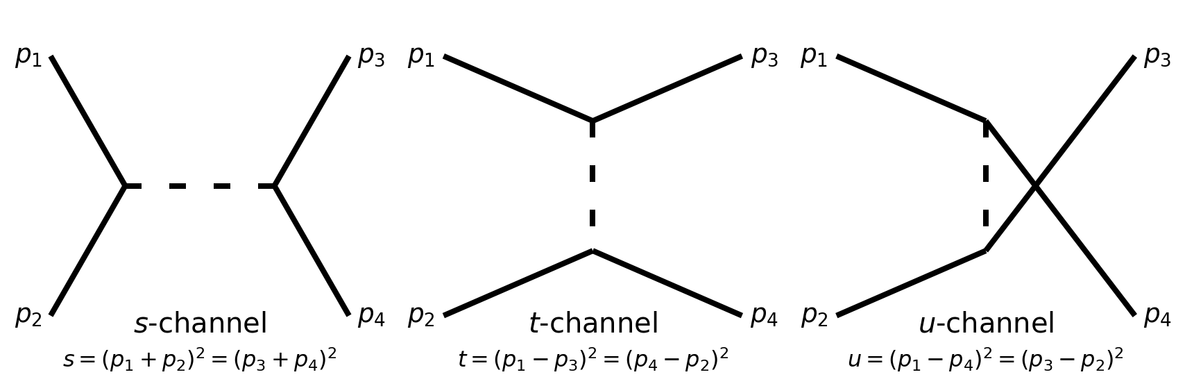
s_channel.text(0.5, 0.08, "$s$-channel", fontsize=15)
s_channel.text(0.5, 0, "$s = (p_1 + p_2)^2 = (p_3 + p_4)^2$", fontsize=12)
s_channel.plot()

t_channel = Diagram(ax[1])
# Vertices
v_p1 = t_channel.vertex(xy=(0.1, 0.7), marker="")
v_p2 = t_channel.vertex(tuple(v_p1.xy), dy=-0.6, marker="")
v_p3 = t_channel.vertex(tuple(v_p1.xy), dx=0.8, marker="")
v_p4 = t_channel.vertex(tuple(v_p3.xy), dy=-0.6, marker="")
v1 = t_channel.vertex(tuple(v_p1.xy), dx=0.4, dy=-0.15, marker="")
v2 = t_channel.vertex(tuple(v_p2.xy), dx=0.4, dy=+0.15, marker="")
# Lines
p1 = t_channel.line(v_p1, v1, arrow=False)
p2 = t_channel.line(v1, v_p3, arrow=False)
interaction = t_channel.line(v1, v2, style="dotted", arrow=False)
e4 = t_channel.line(v2, v_p2, arrow=False)
e5 = t_channel.line(v_p4, v2, arrow=False)
# Labels
v_p1.text("$p_1$", x=-0.06, y=0)
v_p2.text("$p_2$", x=-0.06, y=0)
v_p3.text("$p_3$", x=+0.06, y=0)
v_p4.text("$p_4$", x=+0.06, y=0)
t_channel.text(0.5, 0.08, "$t$-channel", fontsize=15)
t_channel.text(0.5, 0, "$t = (p_1 - p_3)^2 = (p_4 - p_2)^2$", fontsize=12)
t_channel.plot()

u_channel = Diagram(ax[2])
# Vertices
v_p1 = u_channel.vertex(xy=(0.1, 0.7), marker="")
v_p2 = u_channel.vertex(tuple(v_p1.xy), dy=-0.6, marker="")
v_p3 = u_channel.vertex(tuple(v_p1.xy), dx=0.8, marker="")
v_p4 = u_channel.vertex(tuple(v_p3.xy), dy=-0.6, marker="")
v1 = u_channel.vertex(tuple(v_p1.xy), dx=0.4, dy=-0.15, marker="")
v2 = u_channel.vertex(tuple(v_p2.xy), dx=0.4, dy=+0.15, marker="")
# Lines
p1 = u_channel.line(v_p1, v1, arrow=False)
p2 = u_channel.line(v1, v_p4, arrow=False)
interaction = u_channel.line(v1, v2, style="dotted", arrow=False)
e4 = u_channel.line(v2, v_p2, arrow=False)
e5 = u_channel.line(v_p3, v2, arrow=False)
# Labels
v_p1.text("$p_1$", x=-0.06, y=0)
v_p2.text("$p_2$", x=-0.06, y=0)
v_p3.text("$p_3$", x=+0.06, y=0)
v_p4.text("$p_4$", x=+0.06, y=0)
u_channel.text(0.5, 0.08, "$u$-channel", fontsize=15)
u_channel.text(0.5, 0, "$u = (p_1 - p_4)^2 = (p_3 - p_2)^2$", fontsize=12)
u_channel.plot();

References

[1]

K. Peters, “A Primer on Partial Wave Analysis,” arXiv, Dec. 2004, https://arxiv.org/abs/hep-ph/0412069