Since (\(S\) matrix) formulates the transition amplitude from initial state \(\left|i\right>\) to final state \(\left|f\right>\) through \(\left<i\right|S\left|f\right>\), it is a unitary operator—probability is conserved, meaning \(SS^* = I\). Now, having defined the transition operator through \(S = I + iT\), we can introduce another operator: \(K^{-1} = T^{-1} + iI\)[1].
WarningTo do
Explain why this new matrix interesting.
WarningTo do
Definition in terms of \(T\)-matrix.
Special cases of the K-matrix
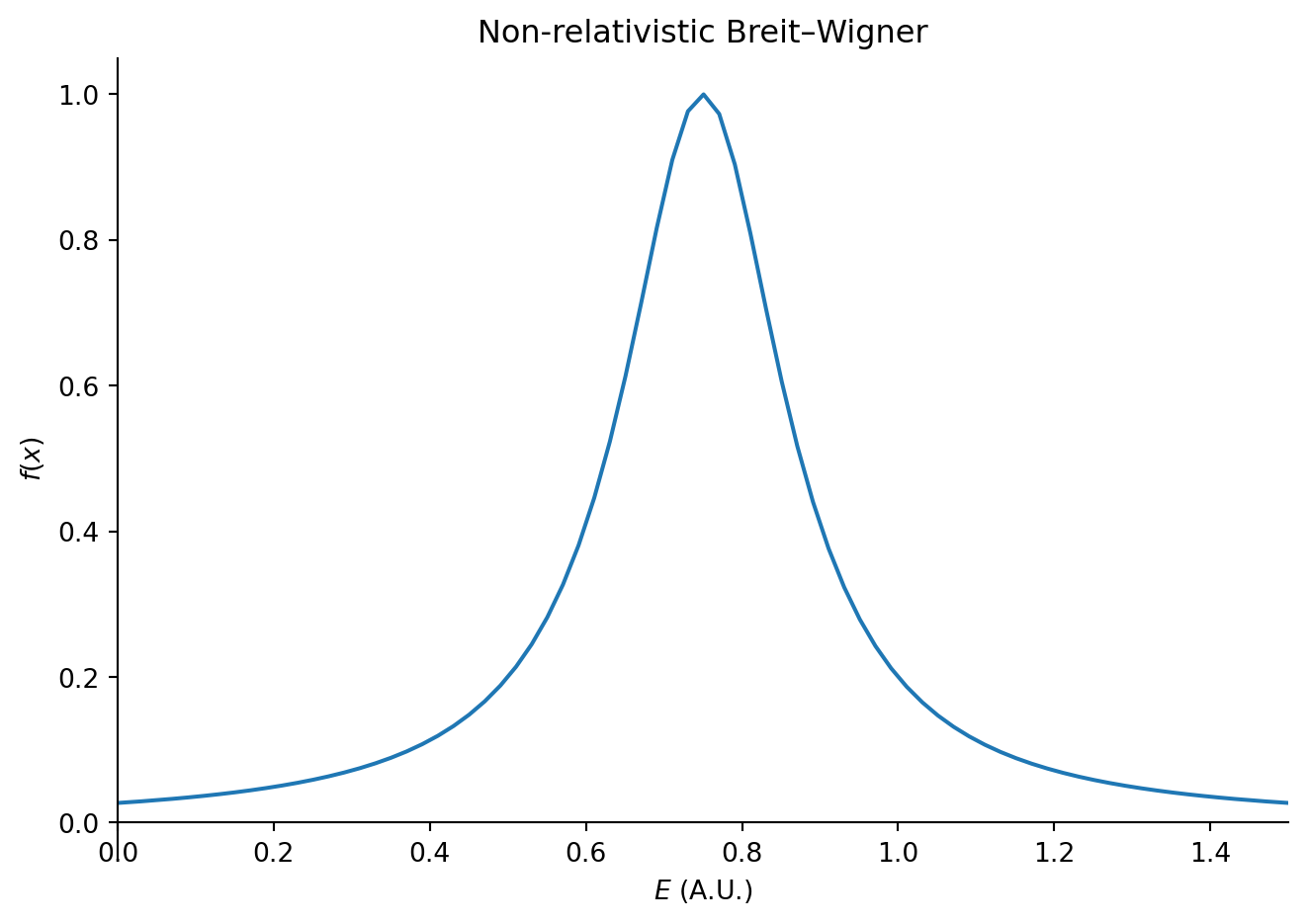
Breit–Wigner
WarningTo do
Derive from \(K\)-matrix instead/as well.
A quantum mechanical state at rest with energy \(E_0\) can be described in terms of the wave function:
\[
\psi(t) = \psi_0 e^{-iE_0t}
\]
Now, if we assume that the state has a decay width of \(\Gamma\), the probability density \(\psi^*\psi\) of this state can be described as:
A particle with a finite decay width can therefore be described as a particle with complex energy:
\[
E' = E_0 - \frac{i}{2}\Gamma
\]
Now, as an experimental physicist, one is interested in predicting the probability of observing the particle at energy \(E\) (we want to describe the observed invariant mass distributions). This can be achieved by applying a Fourier transform, so that \(\psi\) is described in terms of energy \(E\) (or frequency \(\omega\)) instead of time \(t\):
S.-U. Chung, J. Brose, R. Hackmann, E. Klempt, S. Spanier, and C. Strassburger, “Partial wave analysis in 𝐾-matrix formalism,”Annalen der Physik, vol. 507, no. 5, pp. 404–430, May 1995, 10.1002/andp.19955070504.